

\[t \gt 0\]
?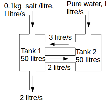
\[x_1, \: x_2\]
respectively.For tank 1
\[\frac{dx_1}{dt}=INFLOW-OUTFLOW=0.1+3\frac{x_2}{50}-2 \frac{x_1}{50}-2 \frac{x_1}{50}=-4 \frac{x_1}{50}+3 \frac{x_2}{50}+0.1\]
.For tank 2
\[\frac{dx_2}{dt}=INFLOW-OUTFLOW=2\frac{dx_1}{dt}-3 \frac{dx_2}{dt}\]
.We can write this in matrix form as
\[\begin{pmatrix} \frac{dx_1}{dt} \\ \frac{dx_2}{dt} \end{pmatrix}= \left( \begin{array}{cc} -4/50 & 3/50 \\ 2/50 & -3/50 \end{array} \right) \begin{pmatrix} x_1 \\ x_2 \end{pmatrix} + \begin{pmatrix} 0.1 \\ 0 \end{pmatrix} \]
We can solve this system by diagonalizing the matrix. First find the eigenvalues. Solve
\[ det \left(\left( \begin{array}{cc} -4/50 & 3/50 \\ 2/50 & -3/50 \end{array} \right) - \lambda \left( \begin{array}{cc} -4/50 & -3/50 \\ 2/50 & -3/50 \end{array} \right) \right)=0\]
\[\begin{equation} \begin{aligned} det \left(\left( \begin{array}{cc} -4/50 - \lambda & 3/50 \\ 2/50 & -3/50 - \lambda \end{array} \right) \right) &= (-4/50 - \lambda )(-3/50-\lambda)- 3/50 \times 2/50 \\ &= \lambda^2+7 \frac{\lambda}{50}+ \frac{6}{2500} \\ &= (\lambda +1/50)(\lambda +6/50) \\ &= 0 \end{aligned} \end{equation}\]
Hence
\[\lambda_1=-1/50, \lambda_2=-6/50\]
.Now find the eigenvectors.
\[\lambda_1=-1/50\]
.\[-1/50 \begin{pmatrix} x_1 \\ x_2 \end{pmatrix}= \left( \begin{array}{cc} -4/50 & 3/50 \\ 2/50 & -3/50 \end{array} \right) \begin{pmatrix} x_1 \\ x_2 \end{pmatrix} \rightarrow \left( \begin{array}{cc} -3/50 & 3/50 \\ 2/50 & -2/50 \end{array} \right) \begin{pmatrix} x_1 \\ x_2 \end{pmatrix} = \begin{pmatrix} 0 \\ 0 \end{pmatrix}\]
Hence
\[-3/50x_1+3/50x_2=0, \: 2/50x_1-2/50x_2=0\]
.We can take
\[x_1=x_2=1\]
then the eigenvector corresponding to \[\lambda_1=-1/50\]
is \[\begin{pmatrix}1\\1\end{pmatrix}\]
.\[\lambda_1=-6/50\]
.\[-6/50 \begin{pmatrix} x_1 \\ x_2 \end{pmatrix}= \left( \begin{array}{cc} -4/50 & 3/50 \\ 2/50 & -3/50 \end{array} \right) \begin{pmatrix} x_1 \\ x_2 \end{pmatrix} \rightarrow \left( \begin{array}{cc} 2/50 & 3/50 \\ 2/50 & 3/50 \end{array} \right) \begin{pmatrix} x_1 \\ x_2 \end{pmatrix} = \begin{pmatrix} 0 \\ 0 \end{pmatrix}\]
Hence
\[2/50x_1+3/50x_2=0, \: 2/50x_1+3/50x_2=0\]
.We can take
\[x1_-3=x_2=2\]
then the eigenvector corresponding to \[\lambda_1=-6/50\]
is \[\begin{pmatrix}-3\\2\end{pmatrix}\]
.The matrix of eigenvectors is
\[P=\left( \begin{array}{cc} 1 & -3 \\ 1 & 2 \end{array} \right)\]
Make the transformation \[\begin{pmatrix} x_1 \\ x_2 \end{pmatrix} = P \begin{pmatrix} u_1 \\ u_2 \end{pmatrix}\]
then the system becomes\[\frac{d}{dt} \left( \begin{array}{cc} 1 & -2 \\ 1 & 3 \end{array} \right) \begin{pmatrix} u_1 \\ u_2 \end{pmatrix} = \left( \begin{array}{cc} -4/50 & 3/50 \\ 2/50 & -3/50 \end{array} \right) \left( \begin{array}{cc} 1 & -2 \\ 1 & 3 \end{array} \right) \begin{pmatrix} u_1 \\ u_2 \end{pmatrix} + \begin{pmatrix} 0.1 \\ 0 \end{pmatrix} \]
Multiply throughout by
\[\left( \begin{array}{cc} 1 & -3 \\ 1 & 2 \end{array} \right)^{-1} = 1/5 \left( \begin{array}{cc} 2 & 3 \\ -1 & 1 \end{array} \right)\]
to get\[\frac{d}{dt} \begin{pmatrix} u_1 \\ u_2 \end{pmatrix} = \left( \begin{array}{cc} -1/50 & 0 \\ 0 & -6/50 \end{array} \right) \begin{pmatrix} u_1 \\ u_2 \end{pmatrix} + \begin{pmatrix} 0.04 \\ -0.02 \end{pmatrix} \]
this is equivalent to the differential equations
\[\frac{du_1}{dt}=-1/50u_1+0.04\]
\[\frac{du_2}{dt}=-6/50u_1-0.02\]
These have the solutions
\[u_1=2+Ae^{-t/50}, \: u_2= -1/6+Be^{-6t/50}\]
We can write this as
\[ \begin{pmatrix} u_1 \\ u_2 \end{pmatrix} = \begin{pmatrix} 2+Ae^{-t/50} \\ -1/6+Be^{-6t/50} \end{pmatrix}\]
Now transform back to
\[x_1, \: x_2\]
.\[\begin{equation} \begin{aligned} \begin{pmatrix} x_1 \\ x_2 \end{pmatrix} &= P \begin{pmatrix} u_1 \\ u_2 \end{pmatrix} \\ &= \left( \begin{array}{cc} 1 & -3 \\ 1 & 2 \end{array} \right) \begin{pmatrix} 2+Ae^{-t/50} \\ -1/6+Be^{-6t/50} \end{pmatrix} \\ &= \begin{pmatrix} 5/2+Ae^{-t/50}-3Be^{-6t/50} \\ 5/3+Ae^{-t/50}+2Be^{-6t/50} \end{pmatrix} \end{aligned} \end{equation} \]
.These solutions can be fitted to any initial conditions to find the constants.